
Explainable AI (XAI) helps you understand and interpret how your machine learning models make decisions. We’re excited to announce that BigQuery Explainable AI is now generally available (GA). BigQuery is the data warehouse that supports explainable AI in a most comprehensive way w.r.t both XAI methodology and model types. It does this at BigQuery scale, enabling millions of explanations within seconds with a single SQL query.
Why is Explainable AI so important? To demystify the inner workings of machine learning models, Explainable AI is quickly becoming an essential and growing need for businesses as they continue to invest in AI and ML. With 76% of enterprises now prioritizing artificial intelligence (AI) and machine learning (ML) over other initiatives in 2021 IT budgets, the majority of CEOs (82%) believe that AI-based decisions must be explainable to be trusted according to a PwC survey.
From our partners:
While the focus of this blogpost is on BigQuery Explainable AI, Google Cloud provides a variety of tools and frameworks to help you interpret models outside of BigQuery, such as with Vertex Explainable AI, which includes AutoML Tables, AutoML Vision, and custom-trained models.
So how does Explainable AI in BigQuery work exactly? And how might you use it in practice?
Two types of Explainable AI: global and local explainability
When it comes to Explainable AI, the first thing to note is that there are two main types of explainability as they relate to the features used to train the ML model: global explainability and local explainability.
Imagine that you have a ML model that predicts housing price (as a dollar amount), based on three features: (1) number of bedrooms, (2) distance to the nearest city center, and (3) construction date.
Global explainability (a.k.a. global feature importance) describes the features’ overall influence on the model and helps you understand if a feature had a greater influence than other features over the model’s predictions. For example, global explainability can reveal that the number of bedrooms and distance to city center typically has a much stronger influence than the construction date on predicting housing prices. Global explainability is especially useful if you have hundreds or thousands of features and you want to determine which features are the most important contributors to your model. You may also consider using global explainability as a way to identify and prune less important features to improve the generalizability of their models.
Local explainability (a.k.a. feature attributions) describes the breakdown of how each feature contributes towards a specific prediction. For example, if the model predicts that house ID#1001 has a predicted price of $230,000, local explainability would describe a baseline amount (e.g. $50,000) and how each of the features contributes on top of the baseline towards the predicted price. For example, the model may say that on top of the baseline of $50,000, having 3 bedrooms contributed an additional $50,000, close proximity to the city center added $100,000, and construction date of 2010 added $30,000, for a total predicted price of $230,000. In essence, understanding the exact contribution of each feature used by the model to make each prediction is the main purpose of local explainability.
What ML models does BigQuery Explainable AI apply to?
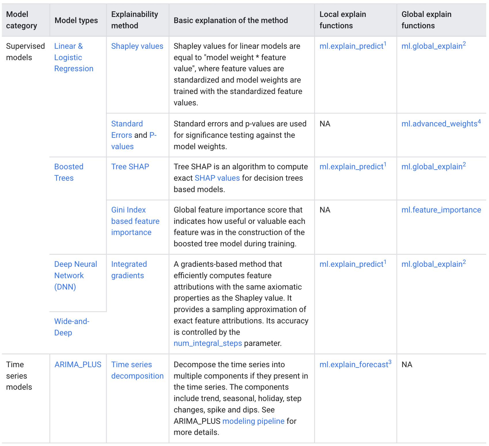
BigQuery Explainable AI applies to a variety of models, including supervised learning models for IID data and time series models. The documentation for BigQuery Explainable AI provides an overview of the different ways of applying explainability per model. Note that each explainability method has its own way of calculation (e.g. Shapley values), which are covered more in-depth in the documentation.
Examples with BigQuery Explainable AI
In this next section, we will show three examples of how to use BigQuery Explainable AI in different ML applications:
Regression models with BigQuery Explainable AI
Let’s use a boosted tree regression model to predict how much a taxi cab driver will receive in tips for a taxi ride, based on features such as number of passengers, payment type, total payment and trip distance. Then let’s use BigQuery Explainable AI to help us understand how the model made the predictions in terms of global explainability (which features were most important?) and local explainability (how did the model arrive at each prediction?).
The taxi trips dataset comes from the BigQuery public datasets and is publicly available in the table: bigquery-public-data.new_york_taxi_trips.tlc_yellow_trips_2018.
First, you can train a boosted tree regression model.
CREATE OR REPLACE MODEL bqml_tutorial.taxi_tip_regression_modelOPTIONS (model_type='boosted_tree_regressor',input_label_cols=['tip_amount'],max_iterations = 50,tree_method = 'HIST',subsample = 0.85,enable_global_explain = TRUE) ASSELECTvendor_id,passenger_count,trip_distance,rate_code,payment_type,total_amount,tip_amountFROM`bigquery-public-data.new_york_taxi_trips.tlc_yellow_trips_2018`WHERE tip_amount >= 0LIMIT 1000000
Now let’s do a prediction using ML.PREDICT, which is the standard way in BigQuery ML to make predictions without explainability.
SELECT *FROMML.PREDICT(MODEL bqml_tutorial.taxi_tip_regression_model,(SELECT"0" AS vendor_id,1 AS passenger_count,CAST(5.85 AS NUMERIC) AS trip_distance,"0" AS rate_code,"0" AS payment_type,CAST(55.56 AS NUMERIC) AS total_amount))

But you might wonder—how did the model generate this prediction of ~11.077?
BigQuery Explainable AI can help us answer this question. Instead of using ML.PREDICT, you use ML.EXPLAIN_PREDICT with an additional optional parameter top_k_features. ML.EXPLAIN_PREDICT extends the capabilities of ML.PREDICT by outputting several additional columns that explain how each feature contributes to the predicted value. In fact, since ML.EXPLAIN_PREDICT includes all the output from ML.PREDICT anyway, you may want to consider using ML.EXPLAIN_PREDICT every time instead.
SELECT *FROMML.EXPLAIN_PREDICT(MODEL bqml_tutorial.taxi_tip_regression_model,(SELECT"0" AS vendor_id,1 AS passenger_count,CAST(5.85 AS NUMERIC) AS trip_distance,"0" AS rate_code,"0" AS payment_type,CAST(55.56 AS NUMERIC) AS total_amount),STRUCT(6 AS top_k_features))
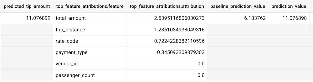
The way to interpret these columns is:
Σfeature_attributions + baseline_prediction_value = prediction_value
Let’s break this down. The prediction_value is ~11.077, which is simply the predicted_tip_amount. The baseline_prediction_value is ~6.184, which is the tip amount for an average instance. top_feature_attributions indicates how much each of the features contributes towards the prediction value. For example, total_amount contributes ~2.540 to the predicted_tip_amount.
ML.EXPLAIN_PREDICT provides local feature explainability for regression models. For global feature importance, see the documentation for ML.GLOBAL_EXPLAIN.
Classification models with BigQuery Explainable AI
Let’s use a logistic regression model to show you an example of BigQuery Explainable AI with classification models. We can use the same public dataset as before: bigquery-public-data.new_york_taxi_trips.tlc_yellow_trips_2018.
Train a logistic regression model to predict the bracket of the percentage of the tip amount out of the taxi bill.
CREATE OR REPLACE MODEL bqml_tutorial.taxi_tip_classification_modelOPTIONS(model_type='logistic_reg',input_label_cols=['tip_bucket'],enable_global_explain=true) ASSELECTvendor_id,passenger_count,trip_distance,rate_code,payment_type,total_amount,CASEWHEN tip_amount > total_amount*0.20 THEN '20% or more'WHEN tip_amount > total_amount*0.15 THEN '15% to 20%'WHEN tip_amount > total_amount*0.10 THEN '10% to 15%'ELSE '10% or less'END AS tip_bucketFROM`bigquery-public-data.new_york_taxi_trips.tlc_yellow_trips_2018`WHERE tip_amount >= 0LIMIT 1000000
Next, you can run <b>ML.EXPLAIN_PREDICT</b> to get both the classification results and the additional information for local feature explainability. For global explainability, you can use ML.GLOBAL_EXPLAIN. Again, since ML.EXPLAIN_PREDICT includes all the output from ML.PREDICT anyway, you may want to consider using ML.EXPLAIN_PREDICT every time instead.
SELECT *FROMML.EXPLAIN_PREDICT(MODEL bqml_tutorial.taxi_tip_classification_model,(SELECT"0" AS vendor_id,1 AS passenger_count,CAST(5.85 AS NUMERIC) AS trip_distance,"0" AS rate_code,"0" AS payment_type,CAST(55.56 AS NUMERIC) AS total_amount),STRUCT(6 AS top_k_features))
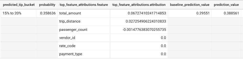
Similar to the regression example earlier, the formula is used to derive the prediction_value:
Σfeature_attributions + baseline_prediction_value = prediction_value
As you can see in the screenshot above, the baseline_prediction_value is ~0.296. total_amount is the most important feature in making this specific prediction, contributing ~0.067 to the prediction_value, though followed by trip_distance. The feature passenger_count contributes negatively to prediction_value by -0.0015. The features vendor_id, rate_code, and payment_type did not seem to contribute much to the prediction_value.
You may wonder why the prediction_value of ~0.389 doesn’t equal the probability value of ~0.359. The reason is that unlike for regression models, for classification models, prediction_value is not a probability score. Instead, prediction_value is the logit value (i.e., log-odds) for the predicted class, which you could separately convert to probabilities by applying the softmax transformation to the logit values. For example, a three-class classification has a log-odds output of [2.446, -2.021, -2.190]. After applying the softmax transformation, the probability of these class predictions is [0.9905, 0.0056, 0.0038].
Time-series forecasting models with BigQuery Explainable AI
Explainable AI for forecasting provides more interpretability into how the forecasting model came to its predictions. Let’s go through an example of forecasting the number of bike trips in NYC using the new_york.citibike_trips public data in BigQuery.
You can train a time-series model ARIMA_PLUS:
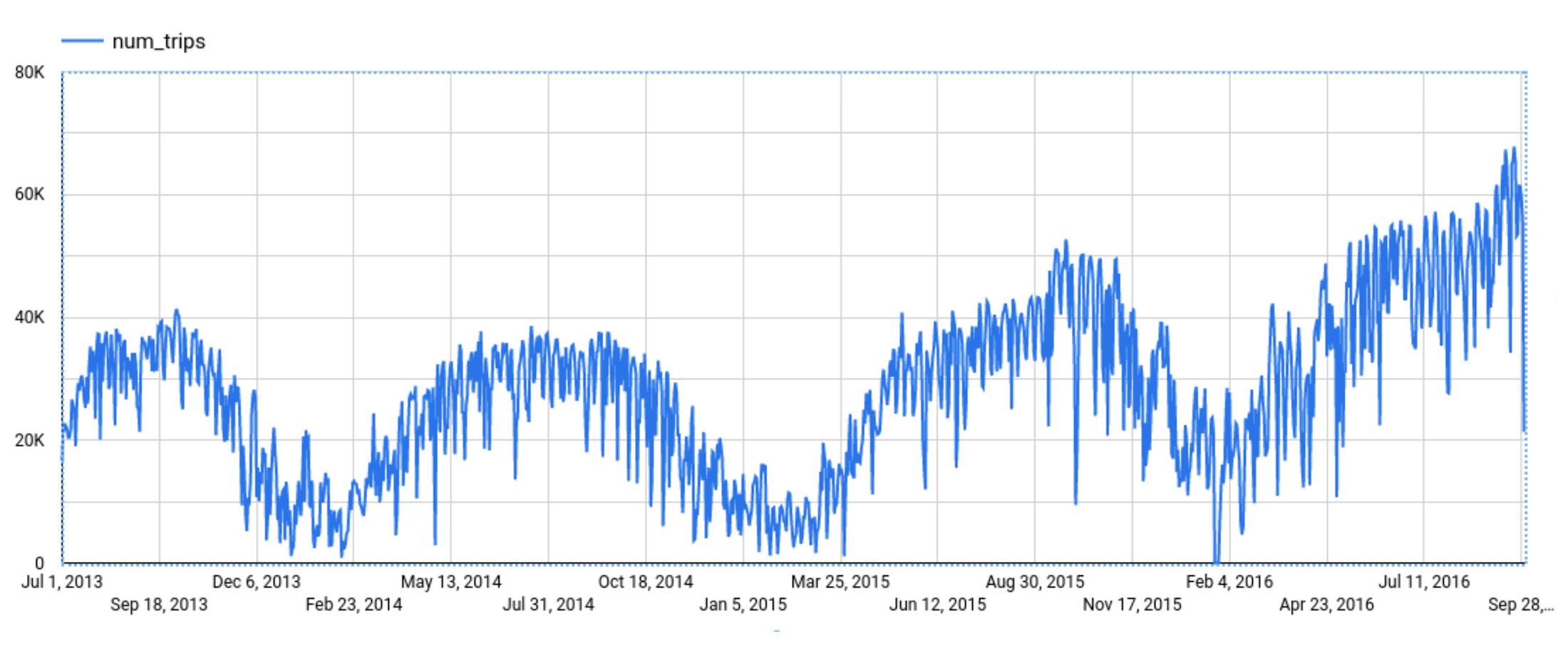
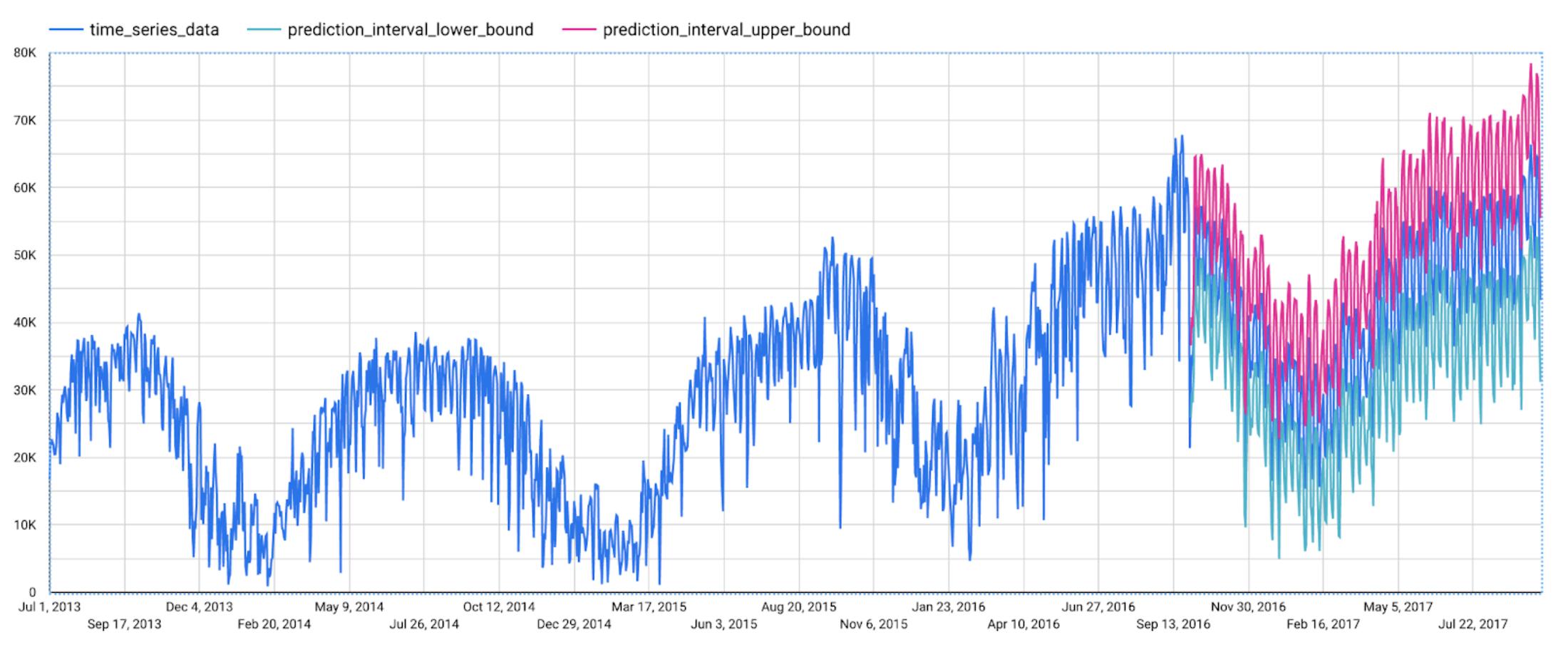
CREATE OR REPLACE MODEL bqml_tutorial.nyc_citibike_arima_modelOPTIONS(model_type = 'ARIMA_PLUS',time_series_timestamp_col = 'date',time_series_data_col = 'num_trips',holiday_region = 'US') ASSELECTEXTRACT(DATE from starttime) AS date,COUNT(*) AS num_tripsFROM`bigquery-public-data.new_york.citibike_trips`GROUP BY dateNext, you can first try forecasting without explainability using ML.FORECAST:SELECT*FROMML.FORECAST(MODEL bqml_tutorial.nyc_citibike_arima_model,STRUCT(365 AS horizon, 0.9 AS confidence_level))
This function outputs the forecasted values and the prediction interval. Plotting it in addition to the input time series gives the following figure.
But how does the forecasting model arrive at its predictions? Explainability is especially important if the model ever generates unexpected results.
With ML.EXPLAIN_FORECAST, BigQuery Explainable AI provides extra transparency into the seasonality, trend, holiday effects, level (step) changes, and spikes and dips outlier removal. In fact, since ML.EXPLAIN_FORECAST includes all the output from ML.FORECAST anyway, you may want to consider using ML.EXPLAIN_FORECAST every time instead.
SELECT*FROMML.EXPLAIN_FORECAST(MODEL bqml_tutorial.nyc_citibike_arima_model,STRUCT(365 AS horizon, 0.9 AS confidence_level))
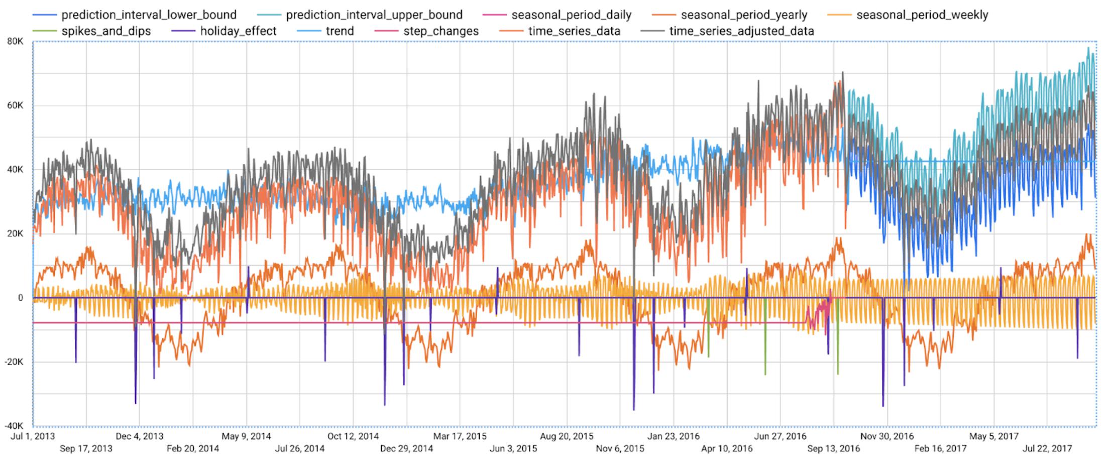
Compared to the previous figure which only shows the forecasting results, this figure shows much richer information to explain how the forecast is made.
First, it shows how the input time series is adjusted by removing the spikes and dips anomalies, and by compensating the level changes. That is:
time_series_adjusted_data = time_series_data - spikes_and_dips - step_changes
Second, it shows how the adjusted input time series is decomposed into different components such as both weekly and yearly seasonal components, holiday effect component and trend component. That is
time_series_adjusted_data = trend + seasonal_period_yearly + seasonal_period_weekly + holiday_effect + residual
Finally, it shows how these components are forecasted separately to compose the final forecasting results. That is:
time_series_data = trend + seasonal_period_yearly + seasonal_period_weekly + holiday_effect
For more information on these time series components, please see the documentation here.
Conclusion
With the GA of BigQuery Explainable AI, we hope you will now be able to interpret your machine learning models with ease.
Thanks to the BigQuery ML team, especially Lisa Yin, Jiashang Liu, Amir Hormati, Mingge Deng, Jerry Ye and Abhinav Khushraj. Also thanks to the Vertex Explainable AI team, especially David Pitman and Besim Avci.
By: Xi Cheng (Software Engineer, BigQuery ML) and Polong Lin (Developer Advocate)
Source: Google Cloud Blog
For enquiries, product placements, sponsorships, and collaborations, connect with us at [email protected]. We'd love to hear from you!
Our humans need coffee too! Your support is highly appreciated, thank you!