
In this three part series we explore the performance debugging ecosystem of PyTorch/XLA on Google Cloud TPU VM. TPU VM earlier this year (2021). The TPU VM architecture allows the ML practitioners to work directly on the host where TPU hardware is attached. With the TPU profiler launched earlier this year, debugging your PyTorch training on TPU VM is simpler than ever before. While the process to analyze the performance has changed, the fundamentals of PyTorch/XLA that you have acquired with the network attached TPU architecture (aka TPU Node architecture), still apply.
In this (first) part we will briefly lay out the conceptual framework for PyTorch/XLA in the context of training performance. Please note that training performance in the current scope refers to training throughput, i.e. samples/sec, images/sec or equivalent. We use a case study to make sense of preliminary profiler logs and identify the corrective actions. The solution to solve the performance bottleneck will be left as an exercise to the reader.
From our partners:
In part-II of this series we will discuss the solution left as an exercise in the part-I and introduce further analysis of the performance to identify other performance improvement opportunities.
Finally, in part-III, we introduce the user defined code annotation. We will see how to visualize these annotations in the form of a trace and introduce some basic concepts to understand the trace.
By the end of this series, we aim to give you a better understanding of how to analyze performance of your PyTorch code on Cloud TPUs and things to consider when working with Cloud TPUs.
Pre-Reading
An understanding of inner workings of XLA Tensor can make the following content more accessible and useful. We encourage you to review this talk from PyTorch Developers Day 2020 and this talk from Google Cloud Next for a quick primer on XLA Tensors. You may also find this article helpful if you are new to PyTorch/XLA. This article also assumes that the reader is familiar with Google Cloud Platform SDK and has access to a Google Cloud project with permissions to create resources such as virtual machines and Cloud TPU instances. Most of the profiler concepts will be explained here, however, introductory reading of TPU VM Profiler is also recommended.
Client-Server Terminology for PyTorch/XLA
As in the TPU Node architecture (before TPU VM) PyTorch XLA still uses the lazy tensor paradigm, i.e. when you are using XLA Tensors, any operations performed on this tensor are simply recorded in an intermediate representation (IR) graph. When a step is marked (xm.mark_step() call), this graph is converted to XLA (HLO format – High Level Operations) and dispatched for execution to TPU runtime (server).
Note that the TPU runtime is the part of TPU server side functionality and all the work done up to the generation of the HLO graph is part of (and henceforth referred to as) the client side functionality. Unlike the previous generation where the TPU runtime (server) was automatically started when you created a TPU instance, incase of TPU VM, PyTorch/XLA library takes care of starting the server when you submit a training. You can also start the XRT (XLA Runtime) server manually on the desired port, Hence the XRT_TPU_CONFIG set in the code snippets later in the post refers to the default port where PyTorch/XLA starts the XRT server. Unlike the previous generation, client and server run on the same host however the abstractions still hold and are helpful to understand the performance (more details here).
Case Study
Context
We will examine UniT (Unified Transformer) training on GLUE/QNLI task using the MMF framework for multi-modal learning from Facebook Research. We will discover an interesting aspect of Multihead Attention Implementation (observed in PyTorch 1.8) that incidentally results in sub-optimal training performance with PyTorch/XLA and discuss a potential corrective action.
Environment Setup
The case study uses TPU VM. In the following steps we create a TPU VM. The following commands can be run from Google Cloud Shell or any machine with the Google Cloud SDK installed and the correct credentials provisioned. (For more details please refer to TPU VM user guide.)
# Set your GCP project id.export PROJECT_ID=<project-id># Modify Zone as applicableexport ZONE=us-central1-agcloud alpha compute tpus tpu-vm create profiler-tutorial-tpu-vm \--project=${PROJECT_ID} \--zone=${ZONE} \--version=v2-alpha \--accelerator-type=v3-8
Once the TPU VM is created and is in READY state, login (ssh) onto the TPU VM host, install TensorBoard profiler plugin and start the TensorBoard server. Please refer to the instructions included in the TPU VM profiler user guide to setup the environment.
gcloud alpha compute tpus tpu-vm ssh profiler-tutorial-tpu-vm \--project ${PROJECT_ID} \--zone ${ZONE} \--ssh-flag="-4 -L 9009:localhost:9009"
Training Setup
We will use two PyTorch environments in the case study beginning with PyTorch 1.8.1 and then move to PyTorch 1.9 as we develop. To ensure PyTorch 1.8.1 as the starting point please execute the following instructions on your TPU VM that was created from the previous section.
sudo bash /var/scripts/docker-login.shsudo docker rm libtpu || truesudo docker create --name libtpu gcr.io/cloud-tpu-v2-images/libtpu:pytorch-1.8.1 "/bin/bash"sudo docker cp libtpu:libtpu.so /libsudo pip3 uninstall --yes torch torch_xla torchvisionsudo pip3 install torch==1.8.1sudo pip3 install torchvision==0.9.1sudo pip3 install https://storage.googleapis.com/tpu-pytorch/wheels/tpuvm/torch_xla-1.8.1-cp38-cp38-linux_x86_64.whl
Update alternative (make python3 default):
sudo update-alternatives --install /usr/bin/python python /usr/bin/python3 100
Configure environment variables:
export XRT_TPU_CONFIG="localservice;0;localhost:51011"
MMF Training Environment
MMF (Multimodal Training Framework) library developed by Meta Research is built to help researchers easily experiment with the models for multi-modal (text/image/audio) learning problems. As described in the case study context we will use the Unified Transformer (UniT) model for this case study. We will begin by cloning and installing the mmf library (specific hash chosen for reproducibility purpose).
git clone https://github.com/facebookresearch/mmfcd mmfgit checkout b771f97adb7f544ed7ffdd02fd486459899c7677
Before we install mmf library in the developer mode, please make the following modifications in the requirement.txt (such that the existing PyTorch environment is not overridden when mmf is installed, to apply the patch copy the text in the following box in a file, e.g. patch-1.txt and run git apply patch-1.txt from the mmf directory.):
diff --git a/requirements.txt b/requirements.txtindex 514d0eb7..7ad34aed 100644--- a/requirements.txt+++ b/requirements.txt@@ -1,5 +1,5 @@-torch>=1.6.0, <=1.9.0-torchvision>=0.7.0, <=0.10.0+#torch>=1.6.0, <=1.9.0+#torchvision>=0.7.0, <=0.10.0numpy>=1.16.6tqdm>=4.43.0,<4.50.0demjson==2.2.4@@ -20,5 +20,5 @@ matplotlib==3.3.4pycocotools==2.0.2ftfy==5.8pytorch-lightning @ git+https://github.com/PyTorchLightning/pytorch-lightning@f79f0f9d-torchaudio>=0.6.0, <=0.9.0+#torchaudio>=0.6.0, <=0.9.0psutil
Apply the following patch (using git apply as explained above) for validate_batch_sizes method (specific to the commit selected for this article):
diff --git a/mmf/trainers/core/evaluation_loop.py b/mmf/trainers/core/evaluation_loop.pyindex 2264f4f5..2af72886 100644--- a/mmf/trainers/core/evaluation_loop.py+++ b/mmf/trainers/core/evaluation_loop.py@@ -10,7 +10,7 @@ from caffe2.python.timeout_guard import CompleteInTimeOrDiefrom mmf.common.meter import Meterfrom mmf.common.report import Reportfrom mmf.common.sample import to_device-from mmf.utils.distributed import gather_tensor, is_master+from mmf.utils.distributed import gather_tensor, is_master, is_xlalogger = logging.getLogger(__name__)@@ -167,6 +167,8 @@ def validate_batch_sizes(my_batch_size: int) -> bool:"""Validates all workers got the same batch size."""+ if is_xla():+ return Truebatch_size_tensor = torch.IntTensor([my_batch_size])if torch.cuda.is_available():batch_size_tensor = batch_size_tensor.cuda()
Install the mmf library in developer mode:
# Running from the mmf base directorysudo -H pip install -e .
Debugging Basics
In order to understand the slow training we try to answer the following three questions:
- Does the number of XLA compilations grow linearly with the number of training steps?
- Does the device to host context switches grow linearly?
- Does the model use any op which does not have an XLA lowering?
To answer these questions, PyTorch/XLA provides a few tools. The quickest way to find these metrics/counters is to enable client side profiling. For a more detailed report you can print metrics_report as explained on the PyTorch/XLA troubleshooting page. PyTorch/XLA client side profiler will often mention one of these metrics in the summary log. Here is an example metrics log:
Metric: CompileTimeTotalSamples: 202Counter: 06m09s401ms746.001usValueRate: 778ms572.062us / secondRate: 0.425201 / secondPercentiles: 1%=001ms32.778us; 5%=001ms61.283us; 10%=001ms79.236us; 20%=001ms110.973us;...Counter: MarkStepValue: 232...Counter: aten::_local_scalar_denseValue: 240...Counter: aten:: <OPS_NAME>Value: 232
It’s helpful to establish an understanding of these metrics and counters. Let’s get to know them.
Debug Metrics
CompileTime Metric
A few important fields to notice here are TotalSamples, Counter, and 50% compilation time. TotalSample indicates how many times XLA compilation happened. Counter indicates overall time spent compilation, and 50%= indicates median completion time.
aten::__local_scalar_dense Counter
This counter implies the number of device-to-host transfers. Once XLA compilation is complete, the execution of the graph is done on the device, however the tensors still live on the device until something in the user’s code does not require the value of the tensor and thus causing the device to host transfer. Common examples of such instances include .item() calls or a control structure in the code which requires the value such as if (…).any() statements. At the execution point when these calls are encountered, if the compilation and execution has not been done, it results in early compilation and evaluation, making training further slower.
aten::<op_name> Counter
This counter indicates the number of instances the said op was seen. The prefix aten:: indicates that cpu/aten default implementation of this op is being used and XLA implementation is not available. Since the Intermediate Representation (IR) graph is to be converted to XLA format and executed on the device, this means that in the forward pass at the instances of these ops, the IR graph needs to be truncated. The inputs to the op are evaluated on device, brought to host and the op is executed with the said inputs. The output from the op is then plugged into the remainder of the graph and execution continues. Based on the number of instances and the location of such ops.
TransferFromServerTime Metric
Total number of samples of this metric indicates the number device to host transfers. In the detailed metric report (torch_xla.debug.metrics.metrics_report()) total time spent in device to host transfers (Accumulator value) and various quantiles are also reported. Client side profiling logs report the count/number of samples only. If this value scales rapidly (rate >=1) with number of training steps, this indicates that there are one or more unlowered ops (aten::*) or constructs fetching tensor values in the model or training code.
Interested readers can find the full list of PyTorch/XLA performance metrics and counters as follows:
import torch_xla.debug.metrics as met# Print all available metrics here# Only metrics with at least one sample appear here# i.e. it will return empty if no IR graph has been created thismet.metric_names()# Print all available countersmet.counter_names()
With the fundamentals discussed thus far, now we are ready to start some experiments to apply the concepts we have learnt.
Experiment-0: Default Run
Once mmf is installed we are ready to start our training of the UniTransformer model on glue/qnli dataset.
export XRT_TPU_CONFIG="localservice;0;localhost:51011"export USE_TORCH=ONpython3 mmf_cli/run.py \config=./projects/unit/configs/all_8_datasets/shared_dec_without_task_embedding.yaml \dataset=glue_qnli \model=unit \training.batch_size=8 \training.device=xla \distributed.world_size=1 \training.log_interval=100 \training.max_updates=1500
Best Practice
Notice that we are using only a single TPU core for the debug run. Notice also that training.log_interval is set to 100. Usually logging involves accessing one or more tensor values. Accessing a tensor value involves a graph evaluation and device to host transfer. If done too frequently it can contribute unnecessary overhead to the training time. Therefore beyond debug/development stage higher logging intervals are recommended.
Observation
Once you execute this training, you will notice logs similar to the following snippet:
2021-07-11T22:42:32 | INFO | mmf.trainers.callbacks.logistics : progress: 1400/1500, train/glue_qnli/loss_0: 0.4457, train/glue_qnli/loss_0/avg: 0.4693, train/total_loss: 0.4457, train/total_loss/avg: 0.4693, experiment: run, epoch: 1, num_updates: 1400, iterations: 1400, max_updates: 1500, lr: 0.00003, ups: 1.06, time: 01m 34s 284ms, time_since_start: 31m 58s 822ms, eta: 01m 40s 714ms2021-07-11T22:44:07 | INFO | mmf.trainers.callbacks.logistics : progress: 1500/1500, train/glue_qnli/loss_0: 0.4457, train/glue_qnli/loss_0/avg: 0.4645, train/total_loss: 0.4457, train/total_loss/avg: 0.4645, experiment: run, epoch: 1, num_updates: 1500, iterations: 1500, max_updates: 1500, lr: 0.00004, ups: 1.06, time: 01m 34s 856ms, time_since_start: 33m 33s 679ms, eta: 0ms
Notice that for 1500 steps the training takes over 33 minutes, updates per sec reported for the final 100 steps is 1.06. Let’s assume you are not impressed with the training speed, and you would like to investigate. Here’s where the PyTorch/XLA profiler can help.
Experiment-1: Enable Client-Side Profiling
PT_XLA_DEBUG environment variable enables the client side debugging functionality, i.e. any part of the user code which can cause frequent recompilations or device to host transfer will be reported during the training and summarized at the end when this functionality is enabled.
export PT_XLA_DEBUG=1export USE_TORCH=ONpython3 mmf_cli/run.py \config=./projects/unit/configs/all_8_datasets/shared_dec_without_task_embedding.yaml \dataset=glue_qnli \model=unit \training.batch_size=8 \training.device=xla \distributed.world_size=1 \training.log_interval=100 \training.max_updates=1500
Observation
Once the client side profiling is enabled, you will notice the following messages starting to appear in your training log:
pt-xla-profiler: TransferFromServerTime too frequent: 36238 counts during 1516 stepspt-xla-profiler: Op(s) not lowered: aten::equal, Please open a GitHub issue with the above op lowering requests.
Notice the logs tagged pt-xla-profiler. The profiler reports too frequent TransferFromServerTime (translation: device to host transfer). Since PyTorch XLA works using the lazy tensor approach, the execution of PyTorch operation graphs it builds and optimizes, is deferred until either a step marker is seen or a tensor value is fetched (device to host transfer) As noted earlier too many of these transfers add to the overhead. 36K occurrences in just 1500 steps is certainly worth investigating. Note that It’s expected to grow with some factor linearly with the number of steps/log_interval, if this factor is greater than number of tensors being captured in the log, it means there are device-to-host transfers beyond what is being logged and it can be reduced to gain performance. This is also why increasing the log interval almost always helps.
Notice also that at the completion of the training (or when training is interrupted once ) the profiler provides further summaries, including a stack trace and frame count (refers to graphs diffs). “Equal” operator with count 9000 appears multiple times and therefore seems to be correlated with high device to host transfers. Notice also “_local_scalar_dense” since it have fewer occurrences, we will investigate it after examining the “equal” op.
WARNING 2021-07-11T22:44:23 | pt-xla-profiler: FRAME (count=9000):WARNING 2021-07-11T22:44:23 | pt-xla-profiler: Unlowered Op: "equal"WARNING 2021-07-11T22:44:23 | pt-xla-profiler: Python Frames:WARNING 2021-07-11T22:44:23 | pt-xla-profiler: multi_head_attention_forward (/usr/local/lib/python3.8/dist-packages/torch/nn/functional.py:4638)WARNING 2021-07-11T22:44:23 | pt-xla-profiler: forward (/usr/local/lib/python3.8/dist-packages/torch/nn/modules/activation.py:980)WARNING 2021-07-11T22:44:23 | pt-xla-profiler: _call_impl (/usr/local/lib/python3.8/dist-packages/torch/nn/modules/module.py:889)WARNING 2021-07-11T22:44:23 | pt-xla-profiler: forward_post (/home/sivaibhav/mmf/mmf/models/unit/transformer.py:442)WARNING 2021-07-11T22:44:23 | pt-xla-profiler: forward (/home/sivaibhav/mmf/mmf/models/unit/transformer.py:509)WARNING 2021-07-11T22:44:23 | pt-xla-profiler: _call_impl (/usr/local/lib/python3.8/dist-packages/torch/nn/modules/module.py:889)WARNING 2021-07-11T22:44:23 | pt-xla-profiler: forward (/home/sivaibhav/mmf/mmf/models/unit/transformer.py:293)WARNING 2021-07-11T22:44:23 | pt-xla-profiler: _call_impl (/usr/local/lib/python3.8/dist-packages/torch/nn/modules/module.py:889)WARNING 2021-07-11T22:44:23 | pt-xla-profiler: forward (/home/sivaibhav/mmf/mmf/models/unit/transformer.py:207)
The stack trace point to the following code from Multihead Attention Implementation:
/usr/local/lib/python3.8/dist-packages/torch/nn/functional.py:4633 if not use_separate_proj_weight:4634 if (query is key or torch.equal(query, key)) and (key is value or torch.equal(key, value)):4635 # self-attention4636 q, k, v = linear(query, in_proj_weight, in_proj_bias).chunk(3, dim=-1)46374638 elif key is value or torch.equal(key, value):
Analysis
Looking up torch.equal manual page reveals:
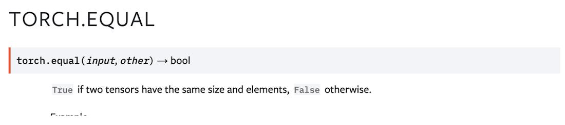
This operator returns a scalar (boolean) value. Using this op in an if statement forces PyTorch/XLA to execute the subgraph leading to this scalar value before it can infer the graph where the boolean value is used. Since this code snippet is part of the forward path, subgraph gets evaluated for every step, as many times as the instances of the .equal operator. And the result of the execution needs to be transferred to the host (device to host transfer) to enable the client to build the rest of the graph. It therefore creates a big bottleneck not only for the overhead of the device to host transfer but also for slowing down the graph building and compilation pipeline. We call such forced evaluations early or premature evaluations.
Note that incase of == operator with tensor operands results in a tensor. == operator itself can become a part of the graph. Therefore using == operator does not result in the early evaluation. However if the value of the resulting tensor affects the resulting graph, i.e. creates a dynamic graph, it can quickly diminish advantages of graph compilation approach with caching (to understand more watch this video).
Potential Corrective Action
We also note that this implementation choice of torch.equal for MHA (MultiHead Attention) serves to optimize resulting GPU kernels, and therefore a good solution to allow this optimization without creating a bottleneck for TPUs is to qualify torch.equal calls with some (non-trainable/configuration) parameter. One potential solution is an implementation similar to this one. However, PyTorch 1.9 code fixed the issue by simplifying the implementation by moving to tensor comparison (is op).
Next Steps
In this post we introduced the basic concepts to understand PyTorch/XLA performance. We also introduced an experiment with a performance bottleneck due to forced execution caused by .equal op. A potential solution in this instance involves the update in the PyTorch core code or update to PyTorch release 1.9. The reader may find these instructions helpful. After the environment is updated, please re-execute the experiment-1 and note the new performance log. In the next part of this article we will review the results and develop further insights into the performance.
Until next time, Happy Hacking! Have a question or want to chat? Find me on LinkedIn.
By: Vaibhav Singh (Machine Learning Specialist, Cloud Customer Engineer)
Source: Google Cloud Blog
For enquiries, product placements, sponsorships, and collaborations, connect with us at [email protected]. We'd love to hear from you!
Our humans need coffee too! Your support is highly appreciated, thank you!